2025 July product update

It’s been some time since our last update but the Qruise team has been hard at work deploying QruiseOS and QruiseML to a host of new users and gathering valuable feedback, which guided most of the new features and bug fixes in this release. These updates are also available on our documentation website, which is now versioned so you can always choose which release of the software you're using to get the most relevant support.

Now let’s dive right into some of the exciting new features that were released in the first half of 2025.

Contents:

• QruiseML
  • New version of qruise-toolset
  • Problem definition
  • Signal Chain and Control Stack
  • Benchmarking
• QruiseOS
  • Use it how you like it
  • New qruise CLI tool
  • Workflow definition improvements
    • Opt-in flags
    • Grouping tasks into subflows

QruiseML

New version of qruise-toolset

A new release (2.2.x) of qruise-toolset is now generally available for all our users. Besides a host of under-the-hood bug fixes, it also updates the interfaces for defining a simulation problem and a control signal. The under-the-hood improvements also led to significant boosts in the performance and efficiency of large-scale simulations.

With this release, several new examples were added to our docs. Existing examples have also been updated to use the latest interface changes.

Problem definition

We introduced a new method remake that allows the user to create a new problem from an already existing Problem by specifying which arguments need to be changed, e.g.

prob = Problem(H, y0, params, (t0, t1))
new_H = Hamiltonian(sigmax() + sigmay())
new_prob = prob.remake(hamiltonian=new_H)

We also introduced a QOCProblem module that's useful for defining optimal control problems. This can now be done using:

prob = QOCProblem(H, y0, params, (t0, t1), yt, loss)
# do the optimisation here
# and get `opt_params`
_, res = solver.evolve(*prob.problem(params=opt_params)[:-1])

This will pass all the variables from prob and use the newly optimised parameters (opt_params instead of params) to the solver.

You can also pass QuTiP Qobj objects as the initial and target states, e.g.

y0 = basis(2, 0)
yt = basis(2, 1)
prob = QOCProblem(H, y0, params, (t0, t1), yt, loss)

Parameters of Array type are now allowed in the Problem definition. Initially, users were prevented from passing arrays of floats as parameters when using Problem. This caused issues in cases where the parameters were intentionally arrays, e.g. when using a PWC pulse or passing matrices A, B, C, and D for a transfer function. We now raise a warning to inform the user of what they're doing, redirecting them to use EnsembleProblem if they want to use an ensemble of scalar values for a specific parameter.

Signal chain and control stack

We introduced a new interface for describing the signal chain and control stack components. The Signal module is now deprecated and we have a new class called SignalChainComponent, which, in its most rudimentary form, has the following structure:

class MyCustomComponent(SignalChainComponent):
   _keys: Tuple = ("key1", "key2")              # necessary parameters
   params: Dict = {"key1": 1.0, "key2": -1.0}   # default values
   # set of parameters that won't participate in the gradient.
   inactive_params: Set = set()

   @staticmethod
   def _gen(t, params, source, name):
      key1 = params[name + "/key1"]
      key2 = params[name + "/key2"]
      return jnp.cos(key1) + jnp.exp(key2)

A Signal chain is not needed anymore. Components get glued automatically thanks to a unified set of parameters and namespace for each component. All the parameters can be put into a ParameterCollection and there are no more any hidden parameters. You can even write complicated chains that share one source but multiple outputs. This is really useful when you want to optimise over the parameters coming from a single source.

A new piecewise constant pulse qruise.toolset.control_stack.PWCPulse has been added which can used to sample from the PWC envelope at a given time t.

Benchmarking

We know that the modelling, simulation, and optimisation tools in QruiseML don’t exist in a vacuum. There are several established open-source tools already used quite widely by the quantum computing community. One of the key features of qruise-toolset is its compatibility with QuTiP which allows you to reuse code from your existing simulations and also voids the need to learn a new interface for defining your system models.

import qruise.toolset as qr
import qutip as qt
omega = 2.0  # TLS frequency
# stationary Hamiltonian, H0
H = qr.Hamiltonian(omega / 2 * qt.sigmaz())

Besides ensuring compatibility with existing tools, we've also benchmarked the software against QuTiP and Dynamiqs, two of the most widely used libraries for scalable quantum dynamics simulation.

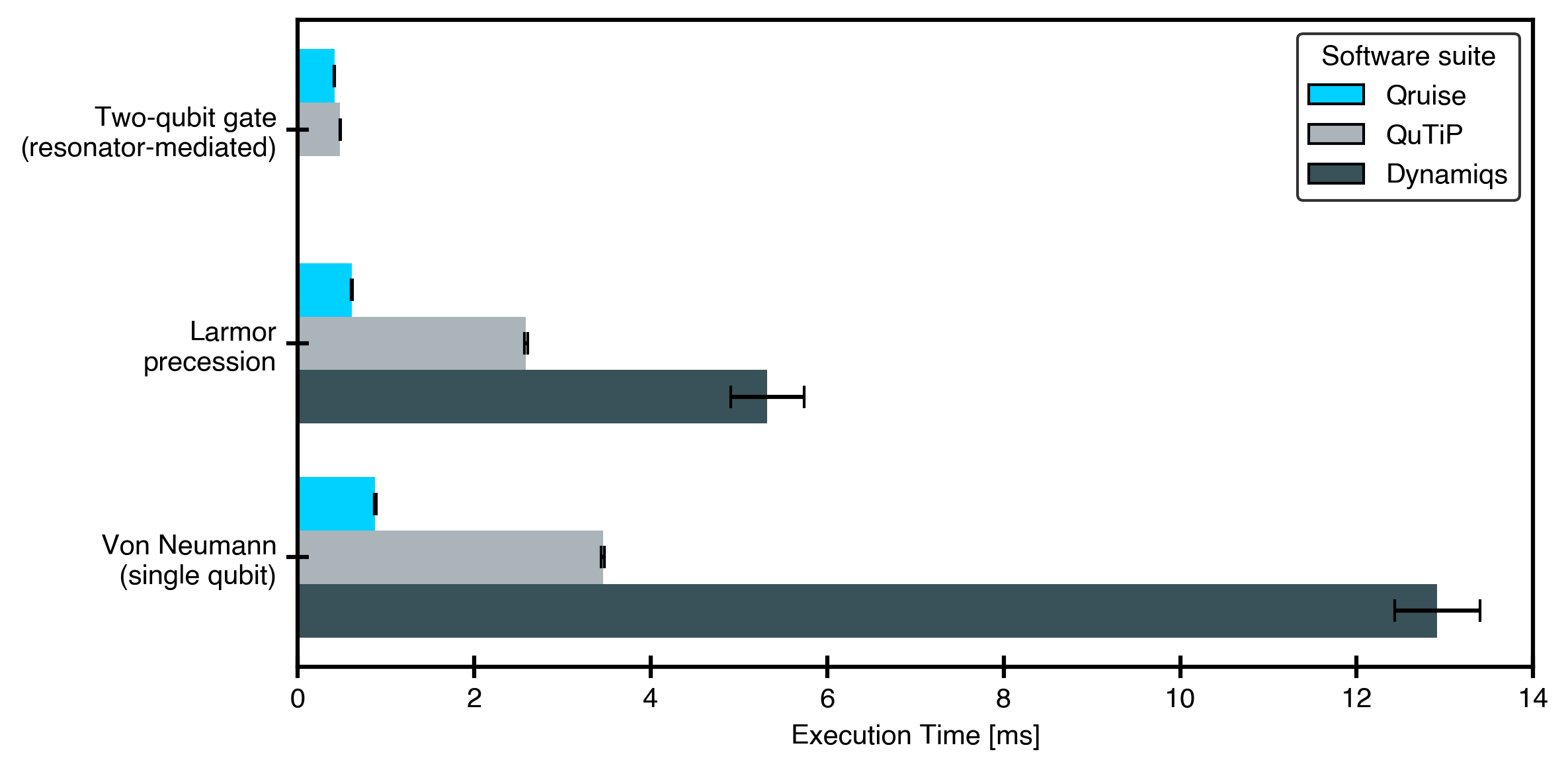
We're happy to report that qruise-toolset performs comparably or significantly better across a wide range of relevant use-cases. A lot of this comes from the underlying JAX library (also used by Dynamiqs). More importantly, we've restructured the internal architecture to ensure efficient implementation (type stability, memory allocations, etc) and to support seamless use of quantum dynamics solvers JAX's automatic differentiation and just-in-time compilation.

We'll release more results in the coming months as we run benchmarks for other use-cases.

QruiseOS

Since the launch of QruiseOS at APS March Meeting 2024, we've had nearly a year of active use by early adopters and long-term users, which provided us with valuable feedback on missing features and nasty bugs. More importantly, we learnt a lot about the diverse ways in which our users expect to interact with the software, which led us to develop new access modes and improved ways to define workflows.

Use it how you like

The users of our software have quite a broad range of preferences when it comes to how they interact with the automated calibration software. In order to address these broad needs, we've made it possible to use QruiseOS through a variety of so-called “front-ends”.

Our canonical browser-based GUI dashboard remains the main entry point for accessing all the different services, triggering workflows, reviewing runs, and inspecting experiment data. We now also have a fully integrated Visual Studio Code and JupyterLab service that lets you interact with all the services through a programmatic python-based SDK right from the comfort of your favourite IDE. Individual users can also load all their extensions and settings into VS Code to get the same experience they're familiar with in everyday programming.

On top of this, we also released a completely new all-purpose command line interface (CLI) tool that's discussed in more detail below.

New CLI tool

A large subset of our users prefer to work from the terminal and we've now launched a comprehensive CLI tool that lets you interact with various QruiseOS services, and run and schedule workflows right from inside your favourite shell.

The qruise command serves as a base for accessing and managing the QruiseOS ecosystem. All features are divided into subcommands bundling related functionalities and following the noun-verb convention. Hence, all calls of the qruise command line have the same basic structure:

$ qruise NOUN VERB ...

where NOUN is a subcommand and VERB is a sub-subcommand. It may sound intimidating at first, but it allows for a very intuitive interface. For instance, you can use the flow subcommand to run and manage flows:

$ qruise flow run   # run a flow
$ qruise flow list  # list all scheduled flows

Similarly, you can use the kb subcommand to interact with the knowledge base:

$ qruise kb log # show the commit history
$ qruise kb commit # commit schema changes
$ qruise kb status # check the status of the knowledge base

You can read more about all the features of the CLI in our documentation.

Workflow definition improvements

Several smaller quality of life improvements have been introduced to how users define bring-up workflows, mostly to facilitate code reuse and boilerplate reduction.

Opt-in flags

When bringing up a QPU, not all tasks require regular execution during everyday operation. Several experiments are only run once after initial cool-down to locate qubits or resonators or identify specific operating points (or regimes). Opt-in flags in the workflow definition files allow you to define specific tasks to be only executed when the specific flag is passed when running the flow. This ensures that you can continue to have a single workflow definition file with all the relevant steps and decide which experiments are run at the time of execution, depending on the state of your QPU.

Grouping tasks into subflows

A bunch of related tasks can be grouped into logical subflows. Besides enabling intuitive navigation between related steps, you can also, for example, re-run a specific subflow until some higher level metric is met. One example use-case is readout optimisation in superconducting qubits, which typically involves iterative execution of a sequence of experiments until the overall readout fidelity reaches the desired value.

Reach out today to request access if you'd like to try out all these new features in QruiseOS and QruiseML!