Updates
April 2026March 2026February 2026January 2026December 2025November 2025October 2025August 2025July 2025May 2025January 2025August 2024March 2026 (v2026.03)
- QruiseML
- Correct super operator construction in
mepwc lindbladpwc_trotterfor large Hilbert spacesremakemethod added toEnsembleProblemEnsembleOptimiserfor robust quantum optimal control- Support for freezing parameters during optimisation
ScipyMinimiserimprovements and fixesScipyMinimiserandOptimistixMinimiserAPIs harmonised- Validate density matrix requirement
c_opsmoved fromlindbladmethods toProblemdefinition- Docs - Unitary gate fidelity and
freeze_keysexamples
- Correct super operator construction in
- QruiseOS
The first flowers are in bloom, and the Qruise team has been busy with spring cleaning in preparation for the months ahead. This release introduces a range of new features, fixes, and improvements across QruiseML and QruiseOS.
QruiseML
You may have noticed that there haven’t been many QruiseML updates recently. That’s because we’ve been working on larger changes that will be released soon. In the meantime, this release includes several fixes and new features for time-evolution equations, problem definitions, and optimisers.
Correct super operator construction in mepwc
In the mepwc method (used for piecewise-constant master-equation simulations), the superoperator used to propagate density matrices was constructed incorrectly. The implementation used unitary.conj().T (the conjugate transpose ) instead of unitary.conj() (the element-wise conjugate ) when forming the Kronecker product representing time evolution, resulting in an incorrect propagator. This has now been fixed.
- return (jnp.kron(unitary, unitary.conj().T) @ y.ravel()).reshape(unitary.shape)
+ return (jnp.kron(unitary, unitary.conj()) @ y.ravel()).reshape(unitary.shape)
lindbladpwc_trotter for large Hilbert spaces
We added lindbladpwc_trotter() as a new Problem method for efficient open quantum system simulation using a first-order Lie–Trotter splitting. This exponentiates only the Hamiltonian for unitary evolution, then applies the dissipator via an explicit Euler step directly to the density matrix. This avoids building and exponentiating the full Liouvillian superoperator used by lindbladpwc(), reducing complexity from to and yielding roughly a speed-up for NV-centre spin systems with . For lindbladpwc_trotter(), the accuracy is first-order in ; for high-precision needs or large time steps, lindbladpwc() remains the recommended choice.
H = qr.Hamiltonian(jnp.pi * jnp.array(qt.sigmax().full()))
c_op = jnp.sqrt(0.1) * jnp.array(qt.sigmam().full())
rho0 = jnp.eye(2, dtype=jnp.complex128) / 2

prob = qr.Problem(H, rho0, {}, (0.0, 1.0), c_ops=[c_op])
solver = qr.PWCSolver(n=50, store=True)
solver.set_system(prob.lindbladpwc_trotter())

*, rhos = solver.evolve(*prob.problem())
remake method added to EnsembleProblem
remake() creates a modified copy of an existing problem while keeping the rest of its configuration unchanged. This is useful when updating parameters, initial states, or time spans without reconstructing the entire problem object.
EnsembleProblem previously inherited remake() from Problem. That implementation rebuilt the object as a Problem, which caused two issues: the returned object was no longer an EnsembleProblem, and list-valued parameters (e.g. {"delta": [0.0, 1.0]}) raised a TypeError. Such parameters are valid in the ensemble context but are rejected by Problem.__init__. EnsembleProblem now implements its own remake() method, which correctly returns an EnsembleProblem and preserves list-valued parameters when creating modified copies.
H = qr.Hamiltonian(jnp.array(qt.sigmax().full()))
y0 = [jnp.eye(2, dtype=jnp.complex128) / 2, jnp.eye(2, dtype=jnp.complex128) / 2]
params = {"delta": [0.0, 1.0]}

ens = qr.EnsembleProblem(H, y0, params, (0.0, 1.0))
new_ens = ens.remake(params={"delta": [2.0, 3.0]}) # returns an EnsembleProblem
EnsembleOptimiser for robust quantum optimal control
EnsembleOptimiser enables robust quantum optimal control by optimising control parameters across an ensemble of physical uncertainties defined in EnsembleProblem. Parameters supplied as Python lists define the ensemble dimensions and are automatically vmapped over (i.e. vectorised across ensemble members using jax.vmap), while scalar parameters are treated as control variables and optimised. EnsembleOptimiser determines this split by inspecting the in_axes metadata returned by EnsembleProblem.problem(): parameters with axis=None are optimised, while parameters with an axis are held fixed. The loss is then computed as a mean over all ensemble members. The API mirrors Optimiser: initialise with a minimiser and solver, call set_optimisation(loss), then run optimise(*ens.problem(), y_t, cartesian=True).
# "delta" as a list → ensemble dimension (vmapped, held fixed)
# "a" as a scalar → control parameter (optimised)
params = {"a": 3.0, "delta": list(jnp.linspace(-5.0, 5.0, 10))}
ens = EnsembleProblem(H, y0, params, (t0, tfinal))
solver = PWCSolver(n=100)
solver.set_system(ens.sepwc())

ens_opt = EnsembleOptimiser(minimiser, solver)
ens_opt.set_optimisation(loss_fn)

opt_params, result = ens_opt.optimise(*ens.problem(), y_t, cartesian=True)
# opt_params contains only control params: {"a": <optimised>}
You can check out EnsembleOptimiser in action for robust optimal control in our NV centre notebook.
Support for freezing parameters during optimisation
We have added an explicit freeze_keys: Set[str] | None = None parameter to Optimiser.optimise() which lets users freeze specific parameters by name to prevent them from being tweaked during optimisation. Frozen parameters are separated before optimisation and correctly preserved in the returned result. A representative example is one where you have a control pulse with drive_freq and drive_amp but only want to optimise the drive_amp. You can now do this with the following approach:
result_params, summary = optimiser.optimise(
    y0=initial_state,
    params={"drive_amp": 0.5, "drive_freq": 5.0},
    t_span=(0.0, 1e-6),
    y_t=target_state,
    freeze_keys={"drive_freq"},
)
EnsembleOptimiser also supports freeze_keys, allowing specific parameters to be held fixed during an ensemble optimisation. Ensemble parameters cannot be frozen because they define the ensemble space, i.e. the parameter values over which the optimiser must remain robust against.
opt_params, result = ens_opt.optimise(
    *ens.problem(),
    y_t=target_state,
    freeze_keys={"sigma"}, # hold sigma constant, optimise all other control params
)
# opt_params["sigma"] == original value (unchanged)
ScipyMinimiser improvements and fixes
ScipyMinimiser also received several improvements.
2D shapes preserved
Array parameters with shape (1, K) (e.g. filter coefficients from TransferFunc) previously lost their 2D structure during flattening, reducing them to 1D and causing an IndexError on reconstruction. Shapes are now captured before flattening and restored correctly.
log_progress and log_interval added
SciPy 1.15 removed the iprint and disp options that previously printed per-iteration loss and gradient norms for L-BFGS-B. ScipyMinimiser now accepts log_progress: bool = False and log_interval: int = 1 to restore similar progress reporting via Python's logging module at INFO level. When enabled, each log entry reports the iteration count, current loss, and gradient norm. The log_interval parameter controls how often progress is reported — for example, if you set it to 5, it will log every fifth iteration.
logging.basicConfig(level=logging.INFO)

minimiser = ScipyMinimiser(
    "L-BFGS-B",
    log_progress=True,  # enable logging of loss + |grad|
    log_interval=5,     # log every 5th iteration
    maxiter=200,
)
# INFO qruise.toolset.optimisers.minimisers - Iteration    5: loss=1.234567e-02  |grad|=3.456789e-04
normalise parameter added
When optimising physical parameters with large magnitudes (e.g. Rabi frequencies ~5×10⁷ Hz), gradient-based methods such as L-BFGS-B can satisfy their gradient tolerance criterion at the very first iteration and terminate without making any progress. The new normalise=True parameter in ScipyMinimiser linearly rescales each parameter to the [0, 1] interval within its declared bounds before optimisation and converts the results back afterwards, improving numerical conditioning. If bounds are omitted, a UserWarning is given when minimise() is called and normalisation is silently skipped.
minimiser = ScipyMinimiser(
   "L-BFGS-B",
   normalise=True,  # rescale parameters to [0, 1] during optimisation
   bounds={"rabi_freq": (0.0, 1e8), "phase": (0.0, 6.28)},
   maxiter=200,
)
ScipyMinimiser and OptimistixMinimiser APIs harmonised
ScipyMinimiser and OptimistixMinimiser now share unified maxiter (maximum iterations) and tol (tolerance) constructor arguments, eliminating the need to use backend-specific parameter names. OptimistixMinimiser no longer hardcodes max_steps=1000; the default still resolves to 1000 when neither maxiter nor max_steps is supplied, but it's now fully configurable. Passing both a unified argument and its native equivalent simultaneously (e.g. maxiter= alongside max_steps=) raises a ValueError to prevent silent conflicts. The minimise() method on both classes no longer accepts **kwargs.
- ScipyMinimiser("L-BFGS-B", options={"maxiter": 500})
- OptimistixMinimiser(optx.BFGS, max_steps=500, rtol=1e-4, atol=1e-4)
+ ScipyMinimiser("L-BFGS-B", maxiter=500, tol=1e-6)
+ OptimistixMinimiser(optx.BFGS, maxiter=500, tol=1e-4)
Validate density matrix requirement
Passing a pure state vector (shape (n,)) as y0 to any density-matrix time-evolution method (lindblad(), von_neumann(), mepwc(), lindbladpwc(), or lindbladpwc_trotter()) previously caused a cryptic IndexError: Too many indices for array during JIT tracing. These methods now validate the initial state shape at call time and raise a clear ValueError if a state vector is supplied instead of a density matrix, indicating the expected shape and suggesting qutip.ket2dm as the standard remedy.
psi0 = jnp.array([1.0, 0.0], dtype=jnp.complex128)  # state vector, not density matrix
prob = qr.Problem(H, psi0, {}, (0.0, 1.0))

prob.lindblad()

# ValueError: lindblad() requires a density matrix of shape (2, 2) matching the
# Hamiltonian dimension, but got shape (2,). For pure states use
# ``from qutip import ket2dm; rho0 = ket2dm(psi0)``; for mixed states
# construct the density matrix directly as a 2D JAX array.
c_ops moved from lindblad methods to Problem definition
Collapse operators for open quantum system evolution (c_ops) are now passed as a keyword argument of Problem.__init__() (and EnsembleProblem.__init__()), rather than as positional arguments of lindblad(), lindbladpwc(), and lindbladpwc_trotter(). This allows type and shape validation to occur once at construction time instead of inside each method.
- prob = qr.Problem(H, y0, params, time_span)
- system = prob.lindbladpwc(c_ops)
+ prob = qr.Problem(H, y0, params, time_span, c_ops=c_ops)
+ system = prob.lindbladpwc()
Docs - Unitary gate fidelity and freeze_keys examples
Section 6 of the spin qubit tutorial extends the existing state-overlap QOC example to gate fidelity optimisation. This is the appropriate metric when designing quantum gates, as it measures unitary closeness for any input state rather than a fixed initial state.
We've also added a new control stack tutorial that demonstrates how to use the freeze_keys feature of Optimiser.optimise().
QruiseOS
The QruiseOS updates mainly focus on improving how workflows and experiments are displayed in the dashboard. We’ve also added OpenCode to help you interact with QruiseOS directly from the JupyterLab environment.
Per-qubit run status
Experiment tasks are now automatically grouped into a single node. Clicking the node opens a page showing each qubit's task sequence side by side, with qubits arranged horizontally and tasks listed vertically in chronological order. This makes it easy to compare progress across qubits and is especially useful for parallelised or multiplexed routines running simultaneously on several qubits.

Full workflow visibility
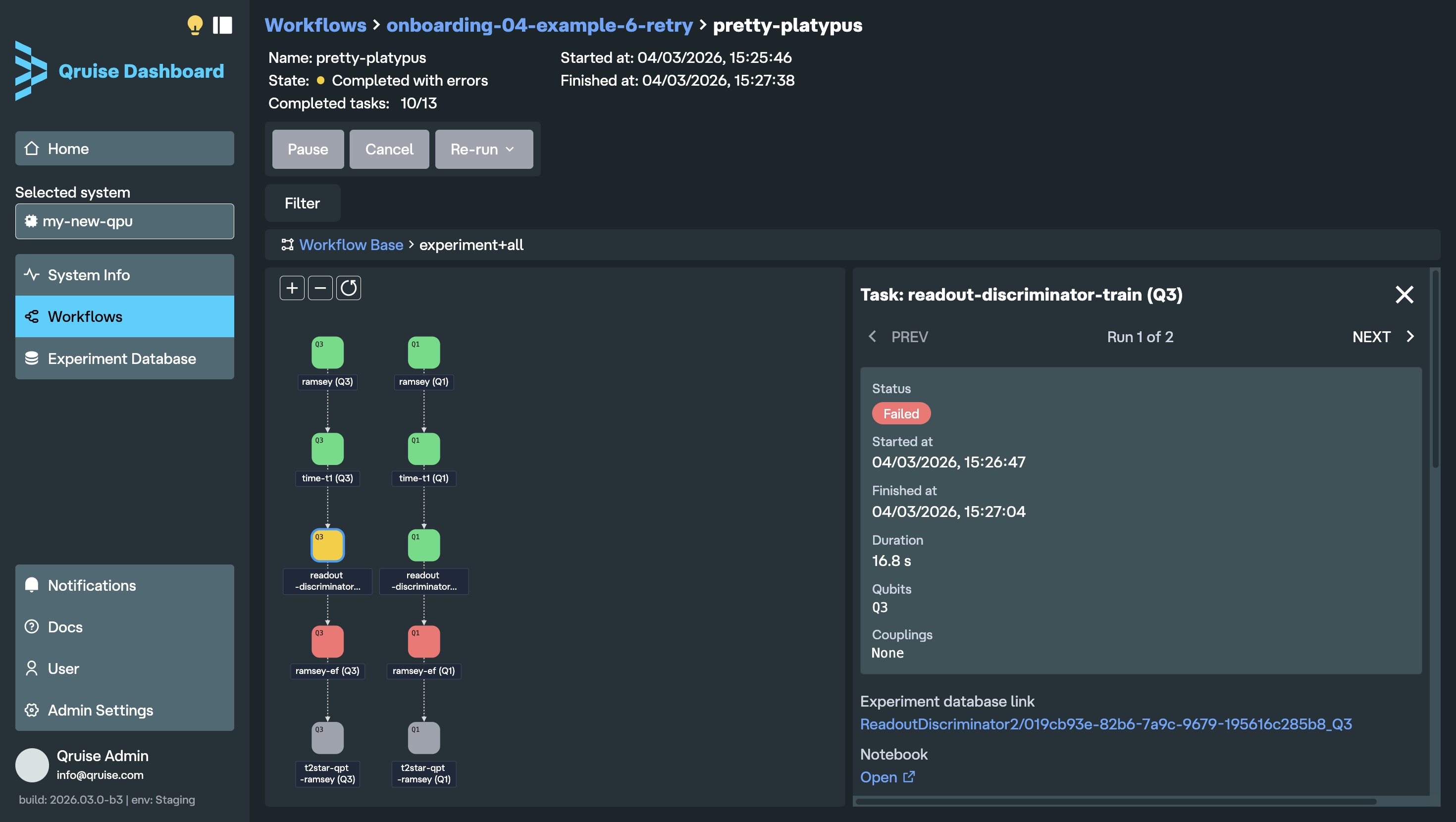
The workflow run view now displays the entire planned workflow from start to finish, regardless of run status. Previously, it only showed tasks up to the current step, so if a workflow failed, later planned tasks were not visible. Each task node is colour-coded by run status: blue (incomplete), pulsing blue (in progress), green (completed successfully), yellow (completed with errors), red (failed), and grey (cancelled, for example due to a failed task earlier in the workflow).
When using the retry function, each run of the retry experiment is shown in the task detail panel, with "PREV" and "NEXT" arrows allowing users to navigate between them.
New subflow icon
Subflows are now indicated with the layers icon. Previously, it was not immediately clear which nodes were tasks and which were subflows (unless of course you clicked on a node to find out). The new icon makes it immediately clear when a node is hiding more tasks (or subflows) inside.
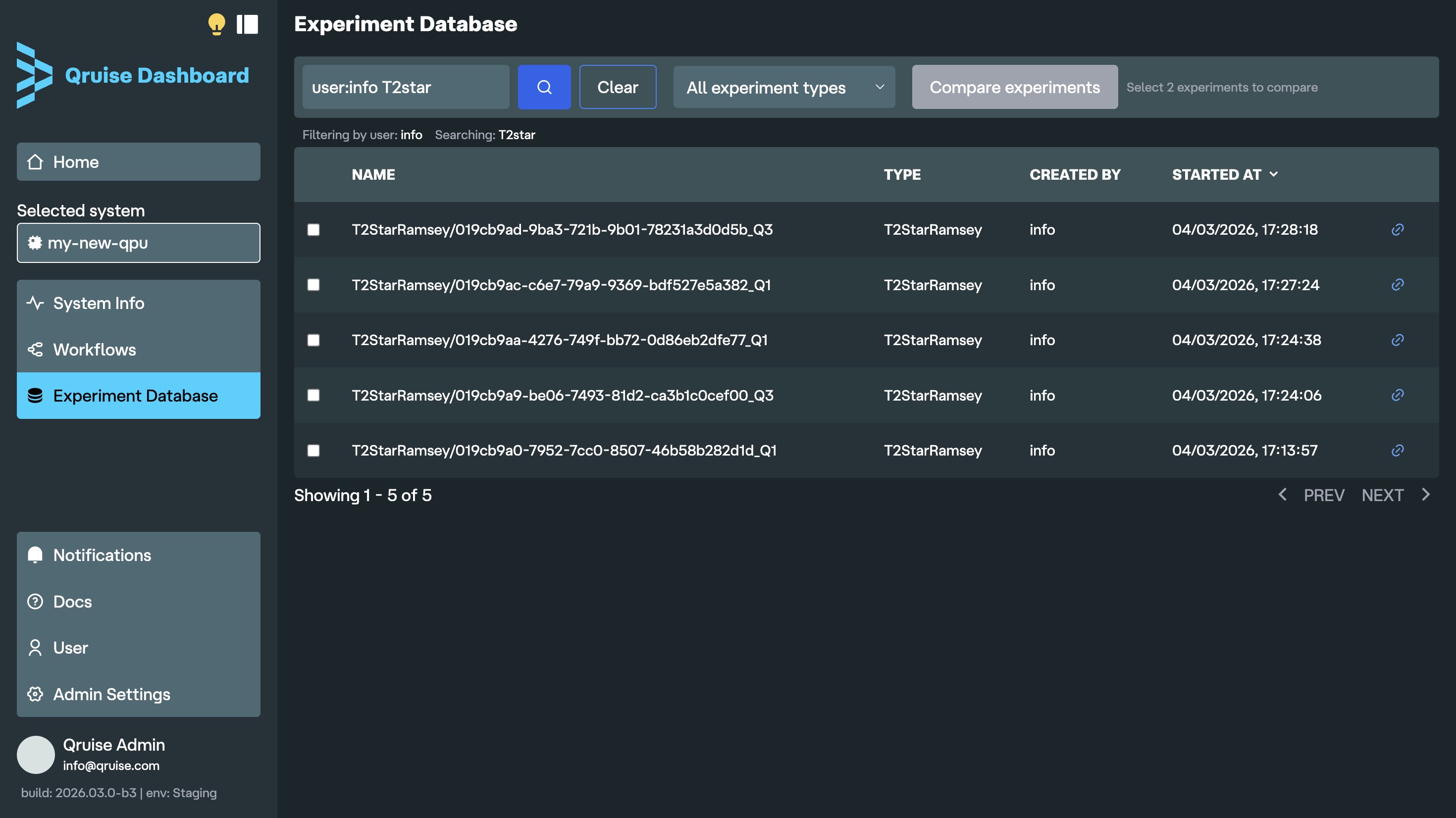
Enhanced search in Experiment Database

Experiments can now be filtered by the user who ran them. No more trying to guess which experiment is yours from the timestamp or by scrolling down long list of KB branches. If you keep an eye on who on your team is getting the cleanest chevrons, you can also see who launched an experiment right next to its type.
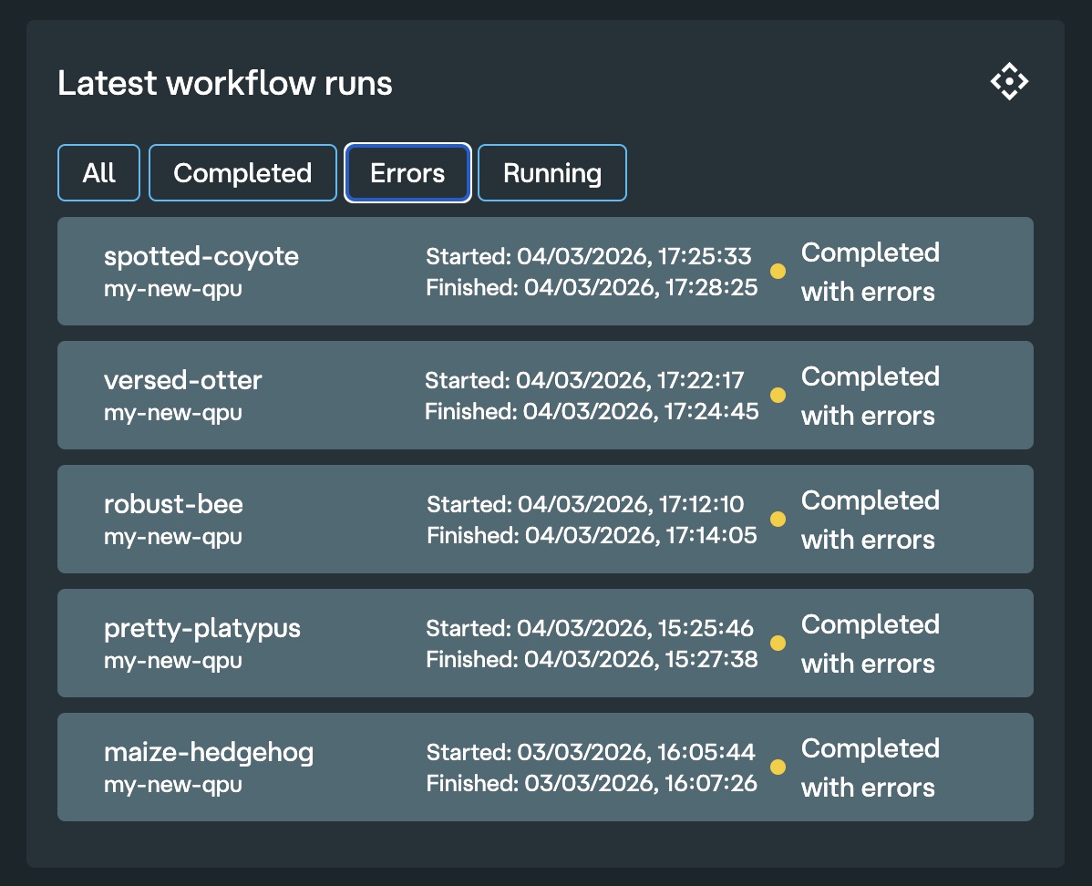
Filter workflows by errors
In the dashboard home, you can now easily filter to show only runs that completed with errors. Hopefully your workflows always complete successfully with no errors, so you never have to use this feature.
Measurement data store integration
Raw experiment data is now stored in the Qruise backend. Previously, data sent to lab hardware (e.g. LabOne Q experiments) was not persisted. Now you can view both the submitted waveform as well as the raw returned data before any postprocessing or analysis. This is particularly useful when trying to debug experiments in the early stages of a QPU bring-up when raw data has a lot of tell-tale signatures about chip issues that might be missed in high level analysis. The data store is tightly integrated with the rest of the QruiseOS stack, allowing you to easily retrieve raw data from the Experiment Database at a later time.
OpenCode + Qruise MCP for natural language interaction

OpenCode is now installed by default in the QruiseOS JupyterLab environment. If you haven't used OpenCode previously, it's an open source agentic AI tool that helps you write software in your terminal, development environment, or desktop. It works seamlessly with the rest of the Qruise stack, including the newly introduced measurement data store. You can ask questions about your Qruise measurements, workflows, and experiment data, and edit workflows directly — for example by adding new experiments or updating your schema — via a Model Context Protocol (MCP) integration, which allows AI assistants to access and interact with QruiseOS. OpenCode comes with free AI models already included and supports most of your favourite LLM providers such as ChatGPT, Copilot, Claude, and Gemini (a separate subscription may be required depending on the model used).
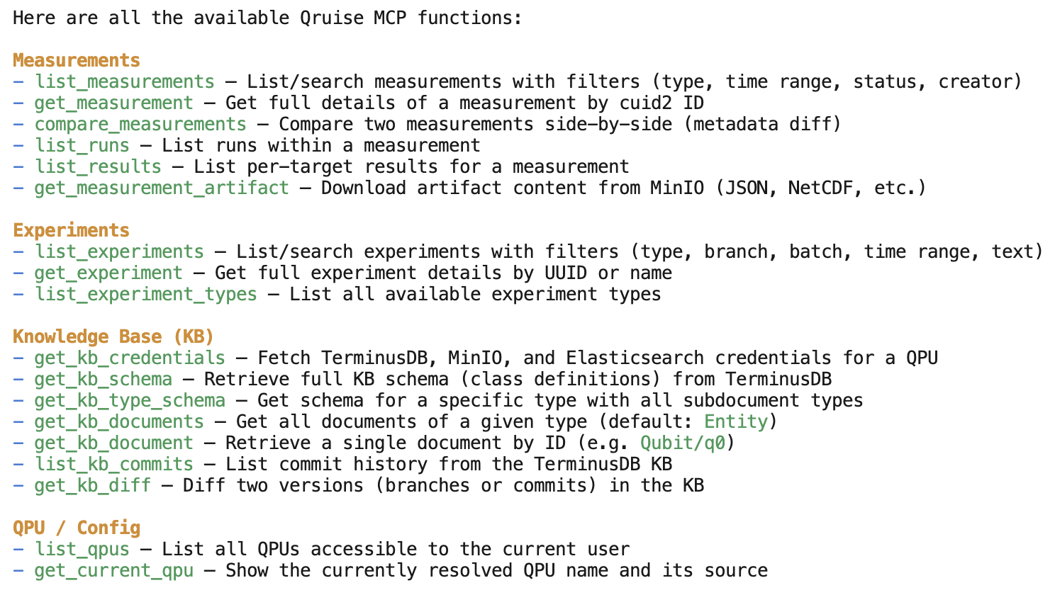
Table of contents
QruiseMLCorrect super operator construction in mepwclindbladpwc_trotter for large Hilbert spacesremake method added to EnsembleProblemEnsembleOptimiser for robust quantum optimal controlSupport for freezing parameters during optimisationScipyMinimiser improvements and fixesScipyMinimiser and OptimistixMinimiser APIs harmonisedValidate density matrix requirementc_ops moved from lindblad methods to Problem definitionDocs - Unitary gate fidelity and freeze_keys examplesQruiseOSPer-qubit run statusFull workflow visibilityNew subflow iconEnhanced search in Experiment DatabaseFilter workflows by errorsMeasurement data store integrationOpenCode + Qruise MCP for natural language interactionStay informed with our newsletter
Subscribe to our newsletter to get the latest updates on our products and services.